Tucanos

Tucanos is a 2D and 3D metric-based adaptation library based on Four-Dimensional Anisotropic Mesh Adaptation for Spacetime Numerical Simulations by Philip Claude Caplan.
The public repository containing the sources can be found here.
This document briefly presents the main theoretical aspects and functionnalities that are offered by this remesher.
Mesh
Metric-based mesh adaptation applies only to simplex meshes, i.e. meshes only composes of simplices. In practice, such elements are triangles in 2D and tetrahedras in 3D.
Simplex meshes
Mesh adaptation can only be applied to conformal meshes made only of simplex elements, i.e. triangles in 2D and tetrahedra in 3D. For other types of meshes, the elements must initially be split into simplices: algorithms for standard elements are given in How to Subdivide Pyramids, Prisms and Hexahedra into Tetrahedra, Julien Dompierre Paul Labbé Marie-Gabrielle Vallet Ricardo Camarero and implemented in tucanos.
Mesh
A mesh consists of
- Vertices
- Elements and element tags
- Tagged faces and face tags
It is characterized by a spatial dimension as well as a cell dimension (3 for tetrahedra, 2 for triangles, ...). The set of mesh entities of dimension is denoted .
A mesh is valid if
- All the elements have a volume ,
- All the faces must be either either
- tagged if
- it belongs to only one element. In this case, they must be oriented outwards
- it belongs to two elements with different tags
- it belongs to more than two elements
- untagged
- tagged if
The mesh also has to be consistent with the geometry (i.e. a CAD-like model) if all the vertices of the tagged faces lie on the corresponding geometry surfaces.
Topology
This module provides data structures and algorithms to represent, build, and query the topological relationships of a mesh. It extracts hierarchical adjacency information from mesh elements (e.g., tetrahedrons, triangles) and faces, mapping out how entities of different dimensions (volumes, faces, edges, vertices) connect to one another.
Core Concepts
Dim: Represents the dimension of an entity (e.g.,0for vertices,1for edges,2for faces,3for volumes).Tag: A unique integer identifier for a specific entity within a given dimension.TopoTag: A tuple of(Dim, Tag)uniquely identifying any topological entity across the entire mesh.- Hierarchy: In this system, "parents" are strictly higher-dimensional entities that bound a "child" entity. For example, a 3D Volume (Dim 3) is a parent to its bounding 2D Faces (Dim 2). A 2D Face is a parent to its 1D Edges.
Core Data Structures
TopoNode
Represents a single topological entity in the mesh and its immediate relationships.
pub struct TopoNode {
    pub tag: TopoTag,            // The unique identifier (Dim, Tag)
    pub children: HashSet<Tag>,  // Tags of lower-dimensional boundary entities (Dim - 1)
    pub parents: HashSet<Tag>,   // Tags of higher-dimensional bounding entities (Dim + 1)
}
Topology
The central registry containing all TopoNodes, categorized by dimension, and caching their hierarchical relationships.
pub struct Topology {
    dim: Dim,
    entities: Vec<Vec<TopoNode>>,
    parents: FxHashMap<(TopoTag, TopoTag), TopoTag>,
}entities: A 2D vector whereentities[d]holds all theTopoNodes of dimensiond.parents: A cached mapping used to quickly find the closest common parent of a given pair ofTopoTags.
MeshTopology
A high-level wrapper that binds a Topology to a specific Mesh instance. It manages the Topology and stores the resolved topological tags for all vertices (vtags).
pub struct MeshTopology {
    topo: Topology,
    vtags: Vec<TopoTag>,
}
API Reference: Topology
Initialization and Serialization
new(dim: Dim) -> Self: Initializes an empty topology supporting up to the specified dimension.from_json(fname: &str) -> Result<Self>: Deserializes a topology from a JSON file and automatically recomputes the parent caches.to_json(&self, fname: &str) -> Result<()>: Serializes the topology to a pretty-printed JSON file.
Querying Tags and Entities
ntags(&self, dim: Dim) -> usize: Returns the number of tags registered in a specific dimension.tags(&self, dim: Dim) -> Vec<Tag>: Returns a list of all tags present in a specific dimension.first_available_tag(&self, dim: Dim) -> Tag: Calculates the next available unique tag for a given dimension (the maximum absolute tag value + 1).get(&self, tag: TopoTag) -> Option<&TopoNode>: Retrieves a reference to aTopoNodeby itsTopoTag.
Hierarchy Construction
insert(&mut self, tag: TopoTag, parents: &[Tag]): Manually inserts a new entity. It automatically updates thechildrenset of the specified parent entities (dimensiontag.0 + 1).get_from_parents(&self, dim: Dim, parents: &[Tag]) -> Option<&TopoNode>: Finds a node in the specified dimension that has the exact set of given parent tags.parent(&self, topo0: TopoTag, topo1: TopoTag) -> Option<TopoTag>: Retrieves the closest common parent of two topology entities, leveraging the internalFxHashMapcache.
Automatic Topology Inference
The module contains robust algorithms to automatically deduce lower-dimensional topology from a mesh's elements and boundary faces:
update_from_elems_and_faces: The primary engine used byMeshTopology. It iterates over the mesh elements and faces, infers the tags for intermediate dimensions (like edges in a 3D mesh), resolves tagging conflicts at corners/junctions (check_and_fix), and returns a fully resolved vector of vertex tags (vtags).clear<F>(&mut self, filter: F): Filters out topology nodes based on a closure, cleaning up dangling child/parent relationships along the way.
API Reference: MeshTopology
new<const D: usize, M: Mesh<D>>(msh: &M) -> Self: Constructs a full topological mapping from a generic meshM. It analyzes element tags (etags) and face tags (ftags), generating unique tags for unmarked internal boundaries, edges, and vertices.topo(&self) -> &Topology: Grants immutable access to the underlyingTopology.vtags(&self) -> &[TopoTag]: Returns a slice containing the computedTopoTagfor every vertex in the underlying mesh, indexed by the vertex ID.
Usage Example
While usually constructed automatically via MeshTopology::new(&mesh), the topology can be constructed manually (which is often useful for testing and custom mesh generation):
let mut t = Topology::new(3);

// Insert a 3D volume (Dim 3, Tag 1) with no parents
t.insert((3, 1), &[]);

// Insert 2D faces (Dim 2) whose parent is the volume (Tag 1)
t.insert((2, 1), &[1]);
t.insert((2, 2), &[1]);

// Insert a 1D edge (Dim 1) bounded by both faces
t.insert((1, 1), &[1, 2]); // Edge shared by Face 1 and Face 2

// Automatically resolve all parent-child hierarchy caches
t.compute_parents();

// Fetch an edge bounded by faces 1 and 2
let edge = t.get_from_parents(1, &[1, 2]).unwrap();
assert_eq!(edge.tag.1, 1);
Geometry
This module provides the structural foundation for associating computational meshes with their underlying geometric domains. It facilitates projecting mesh vertices onto true geometric surfaces (e.g., during mesh adaptation or order elevation), computing geometric deviations (like distance and normal angles), and handling surface curvature.
Core Trait: Geometry<const D: usize>
The Geometry trait defines the essential interface for any geometric representation in a D-dimensional space. It is designed to be thread-safe (Send + Sync).
Key Methods
check(&self, topo: &Topology) -> Result<()>Validates that the geometric model is consistent with the provided topological hierarchy.project(&self, pt: &mut Vertex<D>, tag: &TopoTag) -> f64Projects a given vertexptonto the geometric entity identified bytag. It modifies the vertex coordinates in-place to the projected coordinates and returns the projection distance.angle(&self, pt: &Vertex<D>, n: &Vertex<D>, tag: &TopoTag) -> f64Computes the angle (in degrees) between a given normal vectornand the true geometric normal at the projection ofpton the specified geometric surface.project_vertices<M>(&self, mesh: &mut M, topo: &MeshTopology) -> f64Iterates through all vertices in a mesh and projects boundary vertices (entities with a dimension< D) onto the geometry, returning the maximum projection distance.max_distance<M>(&self, mesh: &M) -> f64Computes the maximum geometric deviation (distance) between the mesh's face/element centers and the true geometry.max_normal_angle<M>(&self, mesh: &M) -> f64Computes the maximum angle deviation between the mesh's discrete normals and the true continuous geometry normals.to_quadratic_triangle_mesh&to_quadratic_edge_meshElevates a linear mesh (straight edges/flat faces) to a quadratic mesh. It achieves this by inserting mid-edge nodes and projecting those new nodes onto the true geometry usingproject_vertices, thereby curving the mesh to match the physical boundaries.
Implementations
1. NoGeometry
A dummy implementation representing the absence of an underlying geometric model.
project()leaves the vertex unchanged and returns0.0.angle()always returns0.0.
2. MeshedGeometry<const D: usize, M: Mesh<D>>
A discrete, STL-like representation of a geometry constructed from a high-resolution boundary mesh. It relies on spatial indices (ObjectIndex, a bounding volume hierarchy) to efficiently find the closest projection points on the discrete surface.
Internal Patch Structures
To manage different topological dimensions, the geometry is split into discrete patches:
MeshedPatchGeometry: Represents a specific topological edge/curve (dimensionD-1). It holds the elements belonging to a specific topological tag and uses a spatial index to compute projections.MeshedPatchGeometryWithCurvature: Represents a specific topological surface patch (dimensionD). In addition to projecting points, it pre-computes and stores principal curvature directions (uand optionallyvfor 3D flows) for anisotropic refinement.
Attributes of MeshedGeometry
patches: A hash map of surface patches, keyed by their topological tag.edges: A hash map of bounding edges/curves, keyed by their topological tag.edge2faces&edge_map: Topological mapping structures.edge_mapmaps the tags of a working simulation mesh back to the original baseline tags of this geometric representation (crucial if the simulation mesh undergoes splitting or re-tagging).
Workflow & Usage
- Initialization: Instantiated via
MeshedGeometry::new(&boundary_mesh). The provided boundary mesh must have correctly tagged faces and edges (e.g., usingmesh.fix()). - Topology Mapping: Use
set_topo_map(&mesh_topo)to reconcile edge tags if the simulation mesh's topology differs slightly from the baseline geometry. - Projection: When
project()is invoked, the geometry inspects the dimension of theTopoTagto route the point:Dim == D: Projects the point onto the corresponding 2D surface patch.Dim == D - 1: Projects the point onto the corresponding 1D boundary curve/edge.Dim == 0: Represents a hard corner/vertex; the point remains fixed in space.
Utility Functions
curvature(&self, pt: &Vertex<D>, tag: Tag)Extracts the principal curvature directions at a specific vertex on a surface patch.write_curvature(&self, fname: &str)Exports the computed curvature vector fields as.vtufiles (appending the topological tag to the filename). This is extremely useful for verifying the curvature field visually in tools like ParaView.
Metric
Metric and Euclidean metric space
An Euclidean metric space is a finite-dimensional vector space where the dot product is defined by means of a symmetric definite positive matrix :
The properties of ensure that it defines a dot product. We will now refer to as a metric tensor or metric.
Canonical Euclidean metric space
The most familiar example of Euclidean space is the one defined by an identity matrix. The 2D canonical one is defined by the 2x2 identity matrix and the 3D by the 3x3 identity matrix .
Geometric definitions in Euclidean spaces
The dot product defined by allows to define the distance notion in . In the following denotes the dimension and is equal either to 2 or 3. We can then define norm and distance definitions:
The length of a segment is then given by the distance between its extremities:
Moreover, given a bounded subset of , the volume is given by:
where is the Euclidean volume of .
Finally, as metric tensor is symmetric, it is diagonalizable. It thus admits the following spectral decomposition:
where is an orthonormal matrix composed of the eigenvectors of :
verifying . is a diagonal matrix composed of the eigenvalues of , denoted , which are strictly positive.
Natural metric mapping
The metric can be seen as a mapping from the unit ball of identity matrix onto the unit ball of , where these unit balls are defined as:
Where denotes the vicinity of point . A visual representation of these unit balls is given in Figure 1. Notice that defines the unit circle in 2D and the unit sphere in 3D.
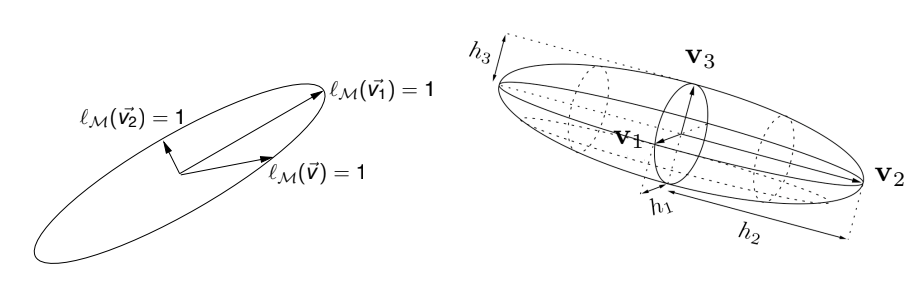
Figure 1: Geometric interpretation of the unit ball of . are the eigenvectors of and are the eigenvalues of . (Loseille 2011)
is defined by the spectral decomposition:
Where denotes a 2D or 3D diagonal matrix. defines the diagonal matrix of the sizes along directions as . This gives the relation between the metric and the size it enforces.
The mapping defined above is written in the form of the following application:
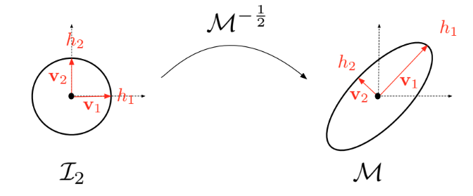
Figure 2: Natural mapping associated with metric . (Loseille 2008)
for more details, see A. Loseille and F. Alauzet, Continuous mesh framework. Part I: well-posed continuous interpolation error, SIAM J. Numer. Anal., Vol. 49, Issue 1, pp. 38-60, 2011. PDF
Riemannian metrics
Riemannian metric space
A Riemannian metric space is defined by a continuous metric field in . The length of an edge is computed using the path where :
The figure below shows length computation in different metric spaces. We see that the iso-values of distance in the Riemannian space are "distorted" with the loss of symmetry when compared to the Euclidean spaces.
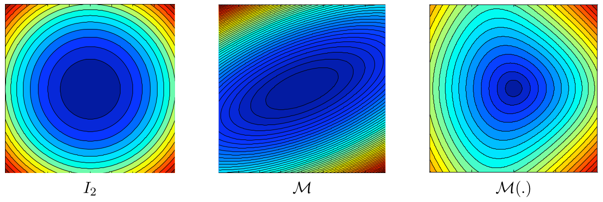
Figure 1: Iso-values of the distance w.r.t canonical Euclidean space (left), euclidean space defined by and Riemannian space defined by (Loseille 2008)
Given a bounded subset of , the volume is given by:
Unit elements and meshes
Let be a simplex element in where denotes its dimension. is unit w.r.t the euclidean metric field when all its edges are equal to 1 in this metric. Mathematically speaking, if we define the list of edges of by , then
And, the volume of is given by:
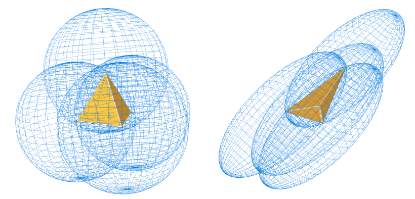
Figure 2: Geometric representation of unit tetrahedrons in metric (left) and an anisotropic metric (right) (Loseille 2008)
The metric for which is unit is unique and referred to as the implied metric of . Conversely, when given a metric , the set of unit elements is not empty. Similarly, the unit notion can be extended to a mesh composed of simplexes with a continuous metric field . The mesh could then be said unit, if all its simplex elements are unit in . However, it is well known that the equilateral tetrahedron does not fill a subset of . Following the proposition in the literature (Loseille 2011), the unit notion for simplex elements is relaxed to the quasi-unit element notion. is said to be quasi-unit if:
Yet, some examples show that elements with a null volume (i.e. degenerated elements) can satisfy the above property. The authors propose a strategy to control the ratio between the volume and the sum of the square length of the edges . This ratio defines the quality function that measures the proximity of to the perfectly unit element in :
The constant is chosen so that is equal to 1 when is perfectly unit in . For a null volume is 0. A constraint on the quality is added to the definition of quasi-unit element to avoid describing degenerated elements.
Then, is said to be quasi-unit if:
Finally, the simplex mesh is said unit with respect to the metric field when all its elements are quasi-unit in . This defines the duality between the discrete and continuous mesh, in the sense that, given a metric field there exists a unit mesh with respect to that metric field .
Complexity
We define the complexity of metric field :
This real value parameter is useful to quantify the global level of accuracy of . It can also be interpreted as the continuous counterpart of the number of vertices of a discrete mesh. There is a direct relationship between the prescribed metric complexity and the number of elements of the generated mesh. Let be a simplex mesh of composed of simplex elements . We can describe this mesh with the metric in which is unit. Then, the continuous mesh complexity and the mesh number of element are linked using the unit element properties:
After remeshing, this relation is not exact because most of the elements are not perfectly unit.
Embedded Riemannian spaces
Two embedded Riemannian spaces have the same anisotropic ratios and orientations. They differ only from their complexity. Mathematically speaking, two Riemannian spaces and are embedded if a constant exists such that:
Conversely, from we can deduce of complexity having the same anisotropic properties (anisotropic orientations and ratios) by considering:
In the context of error estimation, this notion enables convergence order study with respect to an increasing complexity . Consequently, the complexity is also the continuous counterpart of the classical parameter used for uniform meshes while studying convergence.
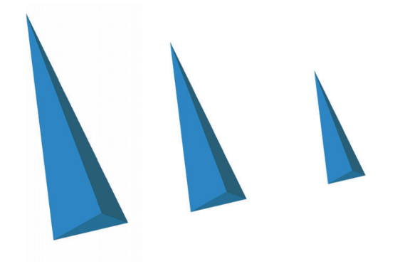
Figure 3: Different unit elements where only the density increases from left to right. (Loseille 2008)
Local decomposition of the metric field in
Let be a metric defined locally on point of domain . Then, by definition, this metric can be written in diagonal form yielding:
In this form, the optimal orientations are given by the rotation matrix and the sizes are given by , given by the eigenvalues . However, we want to write a form that locally decouples the anisotropic information from the global size. Following (Loseille 2011b), the following local parameters can be defined:
- Anisotropic quotients defined as:
- A density defined as:
Locally, the metric writes:
This decomposition is used in the Hessian scaling technique described in the section on Hessian Scaling.
Geometric invariants for unit elements
Unit element's geometric properties can be connected to the linear algebra properties of metric tensors thanks to geometric invariants:
-
Invariant related to the Euclidean volume :
-
Invariant related to the square length of the edges for all symmetric matrix :
Element-implied metric computation
Practically we compute the implied metric by first computing from a two-step transformation. Let be the jacobian transformation matrix from to and be the jacobian transformation matrix from to .
We use the triangle mapping definition to compute and . The element-implied metric becomes:
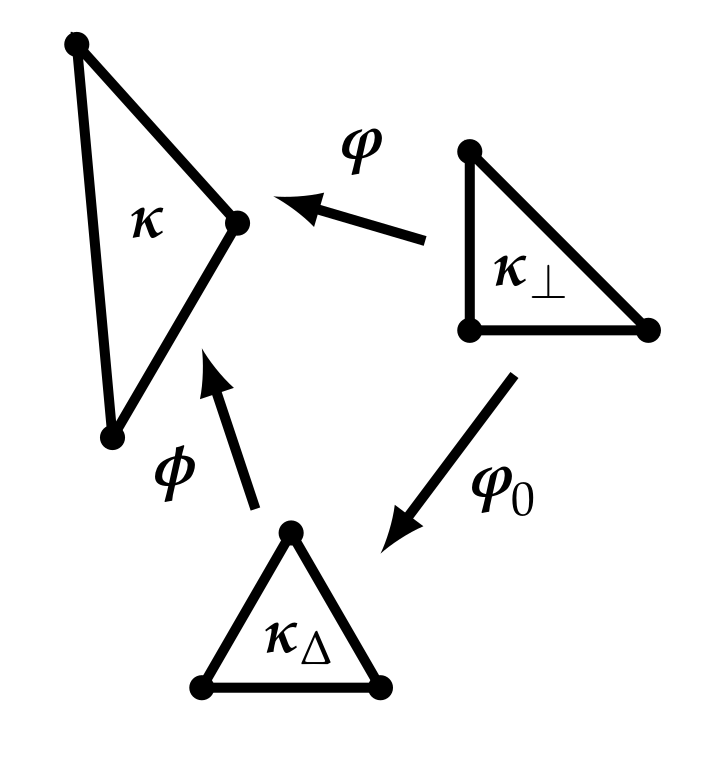
Figure 4: Relationship between the physical and reference elements ( and ) for the calculation of the element-implied metric. (CAPLAN2020102915)
Numerical computation of lengths
Let and be two points of the domain. The length of segment can be numerically approximated using a -points Gaussian quadrature with weights and barycentric coefficients :
where is the metric at the Gauss point. In the context of meshing, we are interested in the evaluation of edge length in the metric. This is a recurrent operation which could be time consuming for the mesh generator. Fortunately, this operation is at the edge level where the metric is known at the endpoints. The problem can thus be simplified by considering a variation law of the metric along the edge and computing analytically the edge length in the metric.
Formally speaking, let be an edge of the mesh of Euclidean length , and and be the metrics at the edge extremities and . We denote by the length of the edge in metric . We assume and we set .
Now, we consider the metric variation law associated with the interpolation operator on metrics.

Logarithmic interpolation is used to interpolate between metrics: as it verifies a maximum principle, i.e. if then for
When interpolating a discrete metric field at is approximated as which is consistent with the assumption of geometric progression of sizes.
Why not linear interpolation?

Linear interpolation between and is given by and does not respect the maximum principle.
As such, logarithmic interpolation is considered along the edge. It can be shown that it is equivalent to a geometric interpolation of the physical length prescribed by the metric F. Alauzet, leading to the following Riemannian distance computation:
Numerical computation of volumes
The evaluation of a tetrahedron volume in a Riemannian metric space consists in computing the volume integral numerically. If a first order approximation in the log-Euclidean framework is considered, we get:
Higher order approximation can be obtained by using Gaussian quadrature. For instance, if one considers a -point Gaussian quadrature with weights and barycentric coefficients , it yields:
Metric operations
Building a metric that is suitable for remeshing may require combining information from different sources or imposing constraints (e.g. minimum or maximum edge lengths, smooth variation with respect to the input mesh, ... ).
Metric Interpolation
In practice, depending on the CFD solver, the metric is either stored on the vertex or the cell center. The definition of an interpolation procedure on metrics is therefore mandatory to be able to compute the metric at any point of the domain. When more than two discrete metrics needs to be interpolated, it is important to use a consistent interpolation framework. For instance, the interpolation needs to be commutative (i.e. the resulting metric does not depend on the order of the interpolation operations between metrics). To that end, the log-Euclidean framework introduced by Arsigny et al. (2006) is used.
Log-Euclidean framework
The authors first define the notion of metric logarithm and matrix exponential. The metric logarithm is defined on the set of metric tensors. For metric tensor , it is given by:
where . The matrix exponential is defined on the set of symmetric matrices. For any symmetric matrix , it is given by:
where . We can now define the logarithmic addition and the logarithmic scalar multiplication :
The logarithmic addition is commutative and coincides with matrix multiplication whenever the two tensors and commute in the matrix sense.
Metric interpolation in the log-Euclidean framework
Let be a set of cell centers and their associated metrics. Then, for a point of the domain such that:
the interpolated metric is defined by:
This interpolation is commutative, but its bottleneck is to perform diagonalizations and to request the use of the logarithm and the exponential functions which are CPU consuming. However, this procedure is essential to define continuously the metric map on the entire domain. Also, since CODA is a cell centered solver and Tucanos is vertex based, this interpolation definition is crucial to get the metric field at the vertexes of the mesh. Moreover, it has been demonstrated (Arsigny et al., 2006) that this interpolation preserves the maximum principle, i.e., for an edge with endpoint metrics and such that then we have:
Metric Intersection
In metric-based adaptation, the metric field computed from the error estimation does not take into account geometric or gradation constraints, that would be defined using different metric fields. Metric intersection is used to get a unique metric field. It consists in keeping the most restrictive size constraint in all directions imposed by this set of metrics.
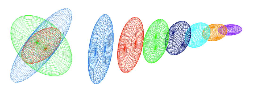
Figure 1: Left, view illustrating the metric intersection procedure with the simultaneous reduction in three dimensions. In red, the resulting metric of the intersection of the blue and green metrics. Right, metric interpolation along a segment where the endpoints metrics are the blue and violet ones. (Loseille 2008)
Formally speaking, let and be two metric tensors given at a point. The metric tensor corresponding to the intersection of and is the one prescribing the largest possible size under the constraint that the size in each direction is always smaller than the sizes prescribed by and . Let us give a geometric interpretation of this operator. Metric tensors are geometrically represented by an ellipse in 2D and an ellipsoid in 3D. But the intersection between two metrics is not directly the intersection between two ellipsoids as their geometric intersection is not an ellipsoid. Therefore, we seek for the largest ellipsoid representing included in the geometric intersection of the ellipsoids associated with and , cf. the Figure above (left). The ellipsoid (metric) verifying this property is obtained by using the simultaneous reduction of two metrics.
Simultaneous reduction
The simultaneous reduction enables to find a common basis such that and are congruent to a diagonal matrix in this basis, and then to deduce the intersected metric. To do so, the matrix is introduced. is diagonalizable with real-eigenvalues. The normalized eigenvectors of denoted by , and constitute a common diagonalization basis for and . The entries of the diagonal matrices, that are associated with the metrics and in this basis, are obtained with the Rayleigh formula:
Remark: and are not the eigenvalues of and . They are the spectral values associated with basis .
Let be the matrix with the columns that are the eigenvectors of . is invertible as is a basis of . We have:
Computing the metric intersection
The resulting intersected metric is then analytically given by:
The ellipsoid associated with is the largest ellipsoid included in the geometric intersection region of the ellipsoids associated with and .
Numerically, to compute , the real-eigenvalues of are first evaluated with a Newton algorithm. Then, the eigenvectors of , which define , are computed using the algebra notions of image and kernel spaces.
See proof
Metric gradation
Metric fields may have huge variations or may be quite irregular when evaluated from numerical solutions that present discontinuities or steep gradients. This makes the generation of a unit mesh difficult or impossible, thus leading to poor quality anisotropic meshes. Generating high-quality anisotropic meshes requires to smooth the metric field by bounding its variations in all directions. It also helps with the convergence of the implicit solver. Mesh gradation (Alauzet, 2010) consists in reducing in all directions the size prescribed at any points if the variation of the metric field is larger than a fixed threshold.
Spanning a metric field
Let be a point of a domain supplied with a metric and the specified gradation. Two laws governing the metric growth in the domain are proposed. In the first one, the metric growth is homogeneous in the Euclidean metric field defined by . The second metric growth is homogeneous in the physical space, i.e., the classical Euclidean space.
The first law associates for any point of the domain a unique scale factor with the metric given by:
With this formulation, each pointwise metric spans a global continuous smooth metric field all over domain parametrized by the given gradation value :
In this case, the resulting metric field grows homogeneously in the Euclidean metric space defined by as the scale factor depends on the length of segment with respect to . As a result, the shape of the metric is kept unchanged while growing. This law conserves the same anisotropic ratio.
For the second law, we associate independently a growth factor with each eigenvalue of , with :
the grown metric at is given by:
The resulting metric field grows homogeneously in the physical space. Indeed, each eigenvalue grows similarly in all directions, as the factor depends only on the distance (in the physical space) from the original point. Consequently, the shape, i.e., the anisotropic ratio of the metric, is no more preserved as the eigenvalues are growing separately and differently. This law gradually makes the metric more and more isotropic as it gradually propagates in the domain.
Alauzet et al. (2021) suggest to mix these two laws to achieve an efficient metric gradation algorithm. For this new law, a growth factor is associated independently with each eigenvalue of :
The authors consider within their numerical examples. For the applications in the work, we will use
Metric reduction
The reduced metric at a point of the domain is given by the strongest size constraint imposed by the metric at and by the spanned metrics (parametrized by the given size gradation) of all the other points of the domain at :
Practical implementation are given in Alauzet (2010).
Thresholds on the local sizes
In order to ensure that the metric field will generate meshes with edge sizes between and , the metric with is modified as with .
Element-implied metric
Given an element , defined by its vertices , the element-implied metric is the metric for which the element is equilateral
If is the jacobian of the transformation from the reference equilateral element to the physical element, the element-implied metric is
In practice is computed as where - is the jacobian of transformation from the reference orthogonal element to the physical element - is the jacobian of transformation from the reference equilateral element to the reference orthogonal element (independent of )
Controlling the step between two metrics
In the remeshing process, it may be interesting to control the step between the element-implied and target metrics. Such control is available within the remesher Tucanos and specified by the parameter .
Given two metric fields and , the objective is to find as close as possible from such that, for all edges :
i.e. to have:
Practically, we define as close as possible as minimizing the Froebenius norm . The optimal is then computed as follows:
- compute ,
- compute the eigenvalue decomposition , with
- compute where ,
- compute .

Figure 2: Representation of the controlled metric by stepping with stepping parameter . The thin blue lines represent and , X. Garnaud
See proof
Metric scaling
- The "ideal" metric is modified using a series of constraints
- Minimum and maximum edge sizes and ,
- Maximum gradation ,
- Maximum step with respect to the element implied metric ,
- A minimum curvature radius to edge lenth ratio (and optionally ), giving a fixed metric
- A scaling is applied, such that the actual metric used for remeshing is
- is chosen to have a given complexity
- A simple bisection is used to compute if all the constraints can be met.
Maths
Notations
- One denotes the Frobenius norm of a matrix by . This norm is associated with the scalar product .
- One denotes by the partial order in the symmetric matrices space : if , i.e. for all , .
Projection on a closed convex subset of the symmetric matrices
The following theorem has been proven in Computing a nearest symmetric positive semidefinite matrix, Higham Nicholas J, 1988:
Theorem 1 Let . Then, is a closed convex subset of the space and then there exists a projection application such that Let and its diagonalisation in an orthonormal basis: , . Then,
Proof
Let and its diagonalisation in a orthonomal basis . As is invariant by linear isometry (, one gets and then the change of variable together with , leads to the following problem This problem can be computed explicitly. Since , ( the canonical basis vectors) This lower bound is reached for the following diagonal matrix , where , and moreover, and is in , which ends the proof.
Generalization
One can generalize the Theorem above as follow:
Theorem 2 Given two symmetric real numbers , let . is a compact convex subset of and then let us denote the associated projection application: Given and its diagonalisation in an orthonormal basis: , . Then,
Proof
The proof follows the one above very closely. The lower bound is got using the inequality: : which is reached for where if , if and otherwise . Again, the matrix is symmetric and indeed in (because since is diagonal, ) and thus is the unique solution of the problem (existence and uniqueness being given by the projection on closed convex sets in a Hilbert space).
Metric optimization problem
Given two metrics . The deformation ratio between a metric and is defined as a function of
The problem.
Given two metrics , and two real numbers , let be the set of metrics which are not to stretched with regard to : Again, this set is compact and convex. Given a matrix norm , we want to find which minimize the distance to , i.e. find such that:
Lemma : Let two metrics > and . The function is bounded and reaches its bounds which are the minimum and maximum of the eigenvalues of . Thus,
Thanks to this lemma, the admissible set can be re-written as
In the -twisted Frobenius norm
First, one studies the case of choosing The above problem reads as follows. Find such that: It is then clear that the change of variable leads to a problem of the form of Theorem 2. Denoting the problem reads find such that Then, from Theorem 2, the solution is and can be computed as follows:
- Compute ,
- Find such that .
- Compute .
- Compute
Remark: Maybe a more suitable formulation would be minimizing the Frobenius norm . This leads to a different problem. For instance, if where . One gets, denoting the error instead of The two distance measures give very different results... does it matter in practice?
Intersection of metrics
Problem.
Given two metrics , we want to find a metric which respects the most restrictive length of and . Moreover, we want that this metric being maximal. More formally, the lenght restriction can be expressed by indeed, is the length of associated with a metric . The local volume associated with a metric is its determinant: , so that the optimization problem reads such that
Solution of the problem.
First, one multiplies by on each side of the constraints, which leads to Then, denoting and applying the change of variable , one gets the simplified problem: such that
This problem can be even more simplified using (does not change the objective as ) and by diagonalization of in an orthonomal basis: Indeed, and , and let us change again the variable , with , the problem is finally: such that
This problem can now be solved explicitly by finding an upper bound. Let such that , then Hadamard inequality provides . Moreover, , from which and then, using the two constraints: , one gets the upper bound reached for the diagonal matrix . Moreover, this matrix is symmetric and verifies and .
Finally, applying the two changes of variables, the unique solution of the problem is
Hadamard inequality
Given a matrix , one has with equality if the are orthogonal.
The result if clear if is singular, if not let , so that one has to show that . is hermitian hence diagonalizable in an orthonomal basis, denoting its eigenvalues, one has
Curvature metric
A metric field can be defined on the boundaries of the computational domain to ensure an accurate representation of the curvature
- the curvature tensor is computed on an accurate geometrical model, giving principal directions and and the associated curvature radii and .
- along direction , a size is imposed (with a given value of , typically )
- along the normal direction the edge length can be chosen arbitrarily. If the representation of the curvature is the only objective, one can chose .
This metric field, defined on the boundary of the computational domain, can then be extended into the domain using a fixed gradation.
boundary-normal size for turbulent boundary layers
For the simulation of turbulent boundary layers, it may be interesting to ensure that the mesh will be fine enough to capture the linear (or log if a wall model is available) layer. In this case, the boundary normal size can be chosen to have a target value of .
In order to estimate the wall shear stress, required to estimate the target edge length in the normal direction, a wall model should be used (as the initial mesh is in practive much too coarse to resolve the turbulent boundary layer).
Optimal metric definition
Feature based adaptation
Feature-based in metric-based adaptation consists in applying the multiscale error estimator in -norm to a scalar function in the domain. This function is denoted as a sensor, or a feature, on which the mesh is adapted to reduce the global interpolation error on this particular sensor, while automatically capturing all scales. In CFD computations, the Mach number is typically used because it captures features of interest such as boundary layers, shocks, and wakes.
Let be a simplex mesh composed of simplex elements . Let be an error model in -norm. The optimal mesh is given by the following minimization problem with constraint :
In the continuous mesh theoretical framework, the goal is to find the optimal continuous mesh which minimizes the given continuous error model for a fixed continuous mesh complexity :
Multiscale error estimator in -norm and feature-based mesh adaptation
Let be a twice derivable smooth function of the state . Let be a simplex mesh on which the function is piecewise linear approximated on elements . The piecewise approximation is defined by the linear interpolate on the mesh . Then, the global interpolation error of in is defined by the -norm of its local interpolation errors, namely:
In (Loseille 2011), the authors prove the existence and unicity of the continuous linear interpolate that defines the continuous linear interpolation error related to the continuous mesh . From corollary 3.4 of (Loseille 2011), the following continuous linear interpolation estimate holds in 2D and 3D:
The continuous linear interpolation model in -norm writes:
Where is a constant depending on the dimension of the simplices composing .
The solution of the problem exists and is given by:
The proofs are given in (Loseille 2011b).
Hessian computation
Tucanos features two methods to compute the Hessian of a given scalar quantity. The first one uses a simple Least-Squares (LS) formulation that is performed twice. The resolution of the Least-squares is carried using a QR decomposition. The second method uses Clément’s L2-projection local operator (L2proj) (Clement, 1975) similarly to the Hessian recovery method presented in (Alauzet, 2021). These methods use the values at the vertices of the mesh, obtained via a volumetric interpolation of the values from the elements to the nodes. This interpolation is performed using the Tucanos library.
Remesher
| Input metric | Adapted mesh |
|---|---|
 |  |
The idea is to perform a series of local modification on an input mesh to have
- edge lengths that are of approximately unit length in the metric space
- element qualities as high as possible
In order to ensure the validity of the final mesh, validity is enforced at each step.
Cavity operators
Remesher implementation: the cavity operator
Given a mesh entity (a vertex or an edge in the present case), the cavity is the set of mesh elements that contain the entity .
A cavity can be filled from a vertex as the set of elements created from and the faces of the boundary of the cavity (oriented outwards).
Edge collapse using cavity operators

The collapse of edge can be performed as follow
- check the tags
- if and , do not collapse
- if and , swap indices and
- build the vertex cavity
- fill the vertex cavity from :
- if passes all the criteria for swaps
- remove all the elements from from the mesh
- insert all the elements from to the mesh
What to do with the metric ?
Edge split using cavity operators

The collapse of edge can be performed as follow
- build the edge cavity
- create the midpoint , project it onto the geometry if needed, and compute the metric
- fill the vertex cavity from :
- if passes all the criteria for swaps
- remove all the elements from from the mesh
- insert verted (with metric ) to the mesh
- insert all the elements from to the mesh
Edge swap using cavity operators

The swap of edge can be performed as follow
- build the edge cavity
- compute
- if is too low, loop over all the vertices on the boundary of C (that are neither nor )
- fill the vertex cavity from :
- if passes all the criteria, it is a valid candidate
- if valid candidates are available, let be the best one (the one with for which the minimum element quality is maximum)
- remove all the elements from from the mesh
- insert all the elements from to the mesh
Smoothing using cavity operators


The smoothnig of vertex can be performed as follow
- build the vertex cavity
- compute
- compute the subset of the vertices in that are tagged in the same entity as or one of its children, and average the positions of these vertices to obtain the new position
- if is on a boundary, project on the geometry
- fill the vertex cavity from :
- if :
- locate the element of that contains (or is the closest), and interpolate the metric in using the barycentric coordinates
- update the location and metric of vertex
The remeshing algorithm
Among Tucanos features is the remeshing algorithm whose goal is to perform operations on the current mesh to inforce as best as possible the desired metric. The objective is to have a mesh that is close to unitary with respect to the prescribed metric.
Practically, if the metric is not defined on the vertices of the mesh, it is interpolated on them using embedded functions from Tucanos. Following that, local operations are performed on mesh entities within cavities (list of geometrical entities containing the entity). Different local operators exists such as edge splits, edge collapses, edge swaps, vertex smoothing etc (Caplan, 2020). Cavity operators function is to replace an existing set of elements by a new one that conserves mesh topology (for example there is no face counted twice). Each local operation is performed if it prescribes edge lengths and element qualities that are quasi-unit. The order of these operations is performed as in the scheduler described in Caplan's PhD (see Figure below). The scheduler is expected to have a significant impact on the outputted mesh. It is believed to be the major source of difference between existing metric-based remeshers such as MMG (mmg), feflo.a (Loseille, 2017) or refine (refine).
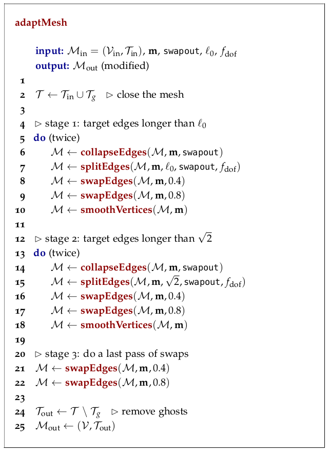
Figure 1: Mesh adaptation scheduling algorithm (Caplan, 2020)